“The Phase Problem”, or, “You didn’t think Mother Nature was gonna let us off that easy, did you?”
Last time we talked about how an incident X-ray beam is scattered by the electrons around atoms, and why the cumulative effect of the scattering is such that the electrons perform the Fourier Transform!
Let’s discuss what this means in practice.
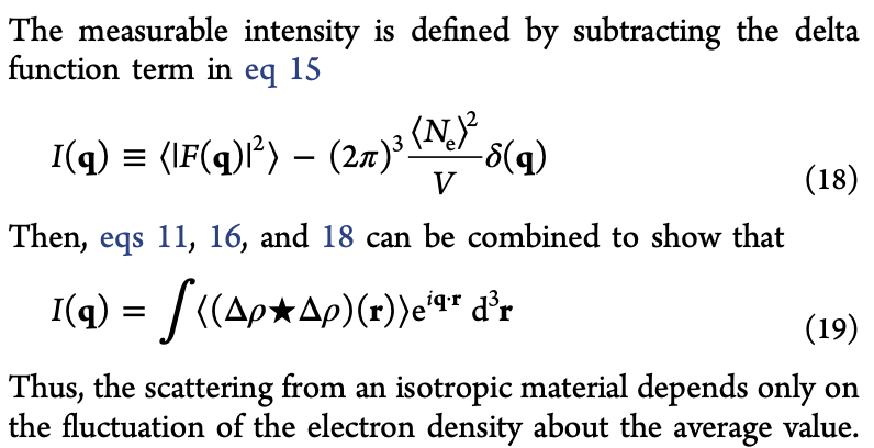
We started with an X-ray wave traveling in a direction, defined by a wavevector, \(\mathbf{k}\).
Electrons scatter that wave, so it radiates out spherically, at all angles defined by \(\mathbf{k}'\) (a vector at an angle \(2\theta\) to the original wavevector, \(\mathbf{k}\))
We choose to express the scattering through the “scattering vector” \(\mathbf{q}\), the vector that points from the tip of \(\mathbf{k}\) to the tip of \(\mathbf{k}'\).
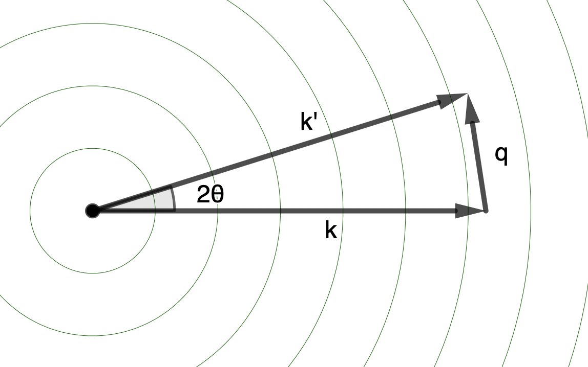
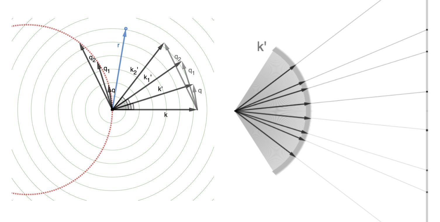
Sweeping through all angles, the collection of these \(\mathbf{k}'\)s forms a sphere.
We measure the projection of this sphere on to an X-ray camera sensor!
Notice that because \(\mathbf{k}\) and \(\mathbf{k}'\) have magnitudes equal to \(2\pi/\lambda\), lower wavelength X-rays (higher frequency, and so higher energy) mean longer wavevectors \(\mathbf{k}\) and \(\mathbf{k}'\), and thus larger-radius spheres swept out by the \(\mathbf{k}\)s.
This will become very important later.
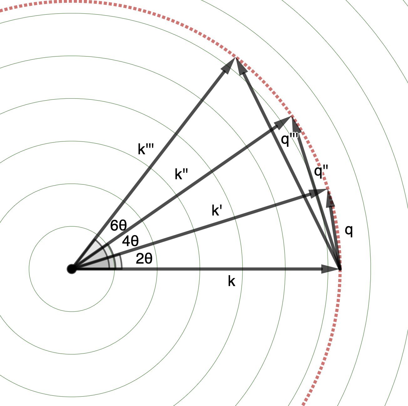
The \(\mathbf{q}\)s sweep out the same sphere, just starting from the tip of \(\mathbf{k}\). (But you should think of all vectors as starting from the origin: in this case, the position of the reference atom/electron.)
Remember: we measure in the \(\mathbf{k}'\) direction, but the interference depends on \(\mathbf{q}\).
The degree of constructive/destructive interference depends on the dot product between the \(\mathbf{q}\)s and the positions of the other electrons (\(\mathbf{r}\)), expressed with the scattering factor \(e^{i \mathbf{q}\cdot\mathbf{r}}\).
Strong interference looks like a bright spot in the far field (right above; and below)
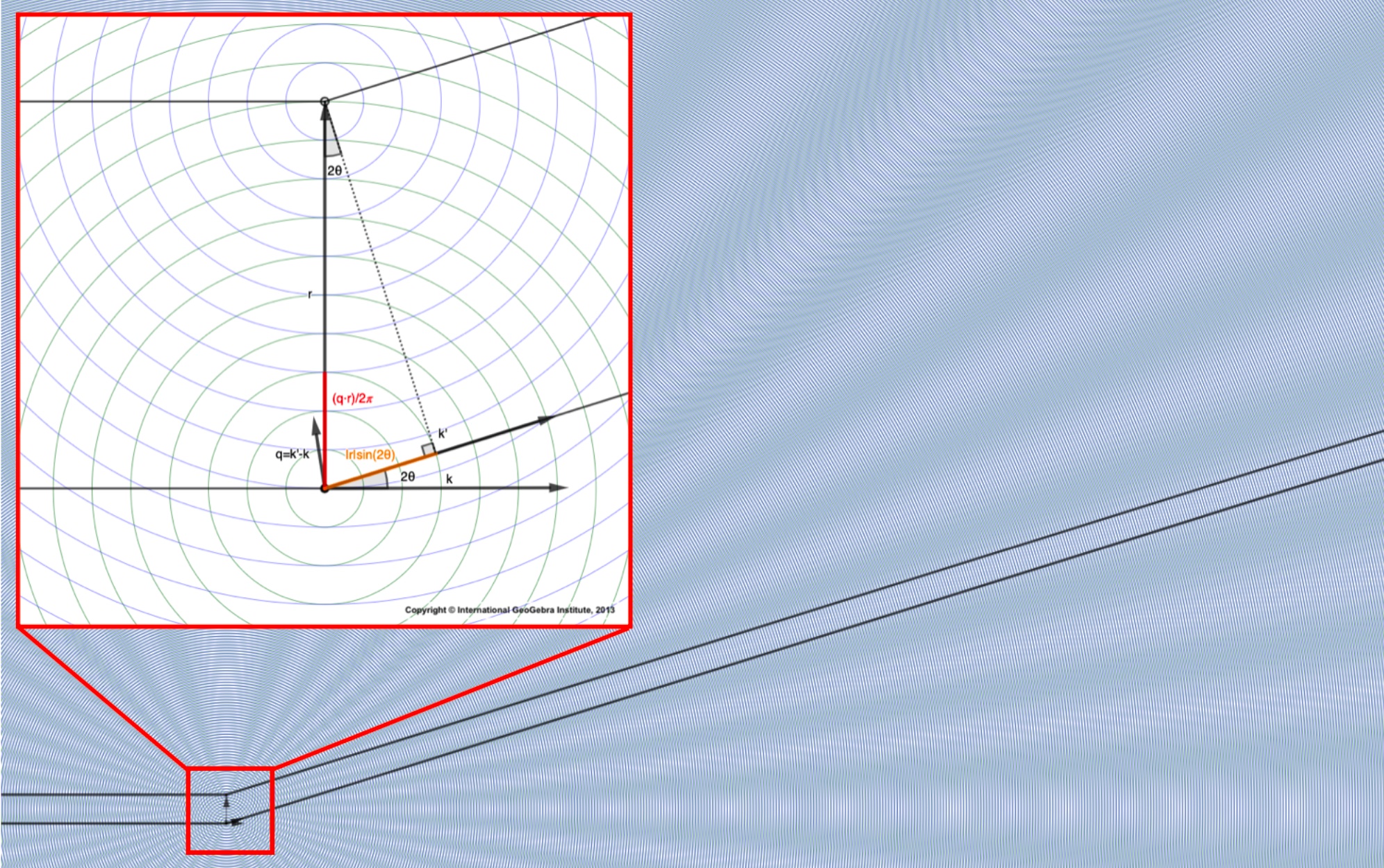
The space of \(\mathbf{q}\)s is called “reciprocal space”, because it has units of reciprocal length.
The Fourier Transform of the electron density lives in this space and, as we saw last time, tells us the cumulative effect (constructive/destructive) of the scattering through the density.
Now, here’s the thing.
These waves are constructively/destructively interfering, i.e. their amplitudes are being added together.
But, if you remember from E&M, we don’t actually measure the amplitude of light waves, we measure the energy they carry, in the form of photons.
The intensity, \(I\) (energy/time) of a light wave is proportional to the amplitude squared.
So if the amplitude, after scattering, at different angles is given by \(F(\mathbf{q})\), what we actually measure is given by:
\[\|F(\mathbf{q})\|^{2}\]
(Not really, but sorta – stick around at the end if you care¹)
Something interesting, as pointed out by Feynman: we don’t actually know this is the correct expression the EM energy density in space. There are actually infinite possible expressions for the energy density, we just choose the simplest one that works…
If we take our def. of \(F(\mathbf{q})\) and square it, we get another Fourier transform!:
\[\|F(\mathbf{q})\|^{2} = \int \int \rho(\mathbf{r})\rho(\mathbf{r}') e^{i\mathbf{q}\cdot(\mathbf{r}'-\mathbf{r})} \mathrm{d}^{3}\mathbf{r} \mathrm{d}^{3}\mathbf{r}' = \int [ \int \rho(\mathbf{u})\rho(\mathbf{r}+\mathbf{u}) \mathrm{d}^{3}\mathbf{u} ] e^{i\mathbf{q}\cdot\mathbf{r}} \mathrm{d}^{3}\mathbf{r}\]
where \(\mathbf{u} = \mathbf{r}'-\mathbf{r}\) is the relative distance between scatterers at \(\mathbf{r}\) and \(\mathbf{r}'\) (notice, we’ve also swapped the labels \(\mathbf{u}\) and \({r}\)).
That expression in brackets being Fourier Transformed is the autocorrelation of the electron density, \(\rho\):
\[(\rho\star\rho)(\mathbf{r}) = \int \rho(\mathbf{u})\rho(\mathbf{r}+\mathbf{u}) \mathrm{d}^3\mathbf{u}\]
This quantity tells you how well correlated (similar) the electron density is with itself, at a displacement \(\mathbf{r}\) away.
Two things to note:
1) This is already very useful!
For example (as we’ll discuss in much greater detail) if the density is periodic ✨ e.g. in a crystal ✨ this autocorrelation will have strong peaks at certain well-defined angles (this is the basis of Bragg’s Law).
Now we can understand why!
A “crystal” is a collection of atoms that repeats. Repeating means it’s a copy of itself, up to translation. This means it’s very autocorrelated at well-defined displacements.
The Fourier Transform (intensity) can then give us information about this!
Back when crystallography was first discovered, it was not obvious that atoms in crystals stayed still enough for crystallography to work as well as it does (if they jiggled around too much, the autocorrelation would be a mess, with no well-defined peaks)
Indeed, Peter Debye purportedly warned Max von Laue that thermal fluctuations would preclude the possibility for constructive interference in crystal diffraction, but von Laue went forward with his experiments anyway.
The rest is history.
2) Because we measure the Fourier Transform of the autocorrelation of the density – not the density itself – we can’t just perform an inverse Fourier Transform on the measured signal to easily recover the density.
:(
That would be nice, but alas…
The cheeky trick that Mother Nature pulls on us here comes from the squaring of the Molecular Form Factor (\(F(\mathbf{q})\)).
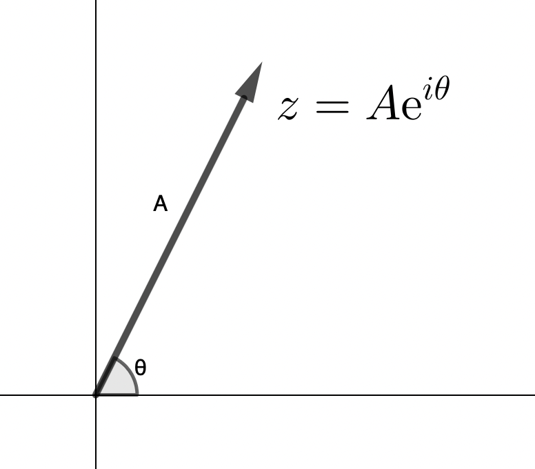
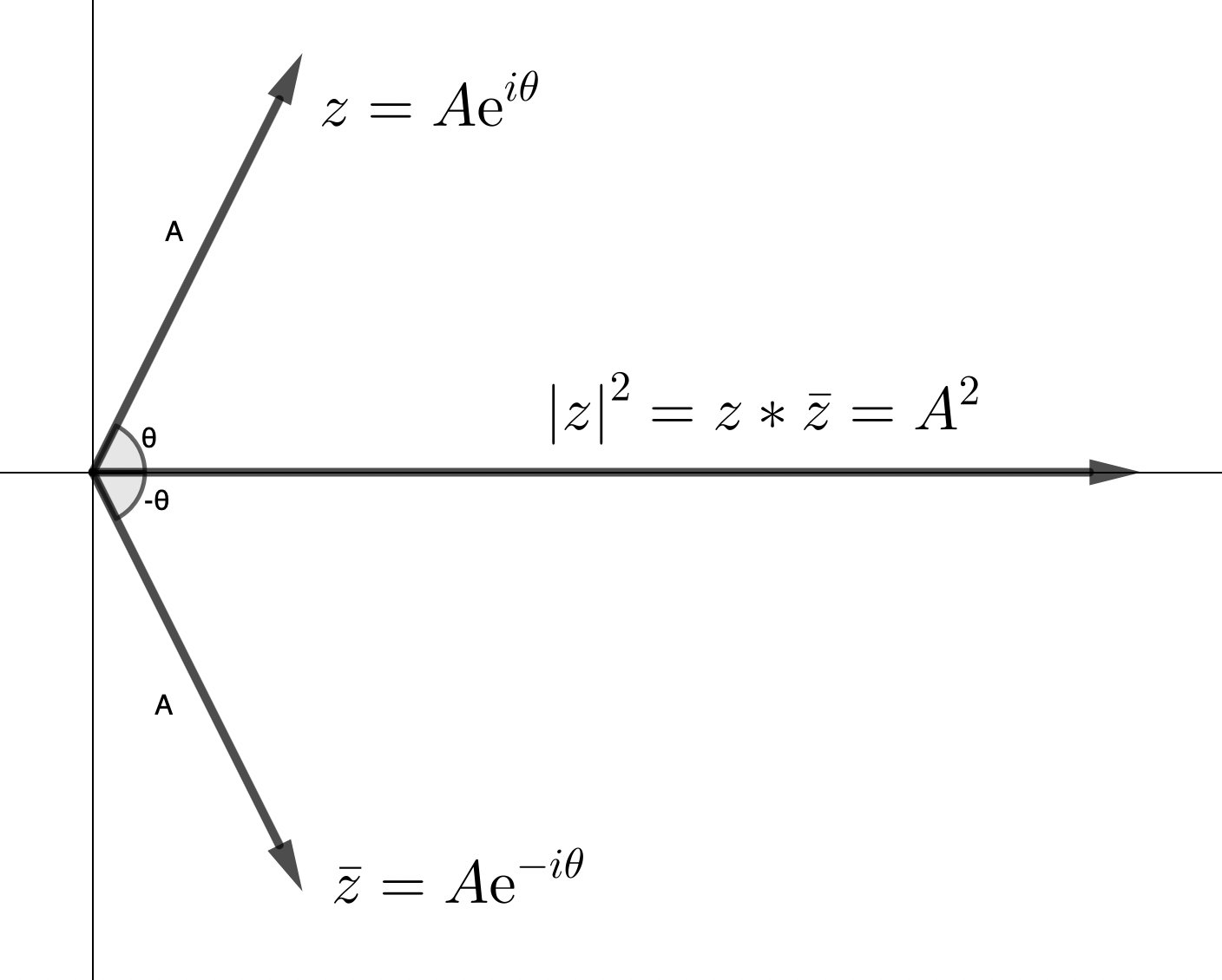
See, the Fourier transform outputs complex numbers, and complex number have an amplitude (\(A\)) and a phase (\(\phi\)):
\[z = Ae^{i\phi}\]
When you want to get the magnitude of a complex number you take the “modulus”, which means multiplying by the “complex conjugate” (the complex number w/ the same amplitude, but opposite phase) – this gives you the magnitude of the complex number squared (\(\|z\|^{2}\)):
\[\|z\|^{2} = z z^{\ast} = Ae^{i\phi} * Ae^{-i\phi} = A^{2}\]
You lose all information about the phase (\(\phi\)). You only get information about the amplitude (\(A\)).
The amplitudes still give you a lot of information, but to truly recover the electron density from the data we collect, we need to get those phases.
This issue is named the “phase problem” in crystallography (for, hopefully, obvious reasons).
I hope, at this point, you’re getting some glimpse of the game were playing here with X-ray crystallography.
We’ve already partially answered a few key questions, e.g.:
-
Why X-rays?
-
Why crystals?
But we’ve really only just begun.
The beauty of this method (and the magic in it, still to be discovered) is going to become clear when we dive in to how things change when we build the crystal periodicity in to our theory.
Lots of fun stuff to come!
But for now, be well.
Part 3 here
¹What we actually measure is the average autocorrelation of the variation of the density about the mean.
The scattering from the average density comes out of the total scattering as a peak in the center of the beam.