“The Ewald Sphere”
If you need enticement to stick with this – this is probably the most beautiful piece of theory I’ve ever come across ✨it’s really something special.
Last time, we found that when an X-ray beam scatters through a volume of electron density, the intensity we measure in the far field is proportional to the squared magnitude of the form factor:
\[I(\mathbf{q}) \propto \| F(\mathbf{q}) \|^{2}\]
Let’s review a little…
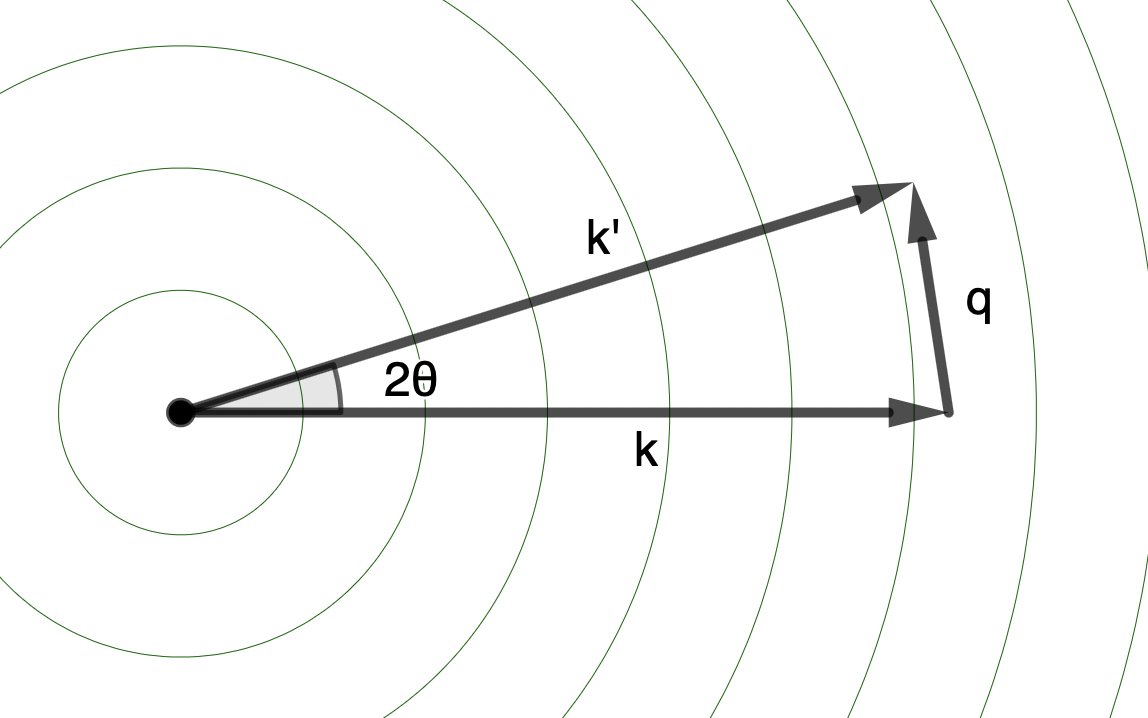
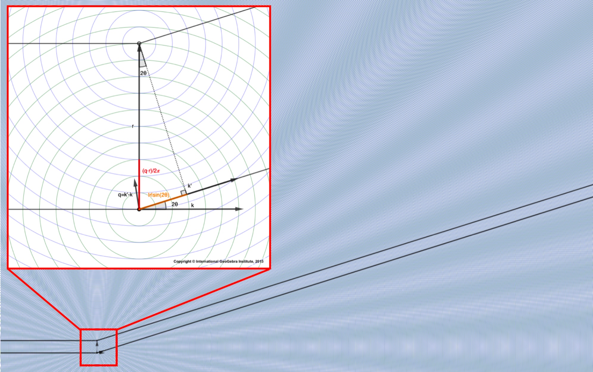
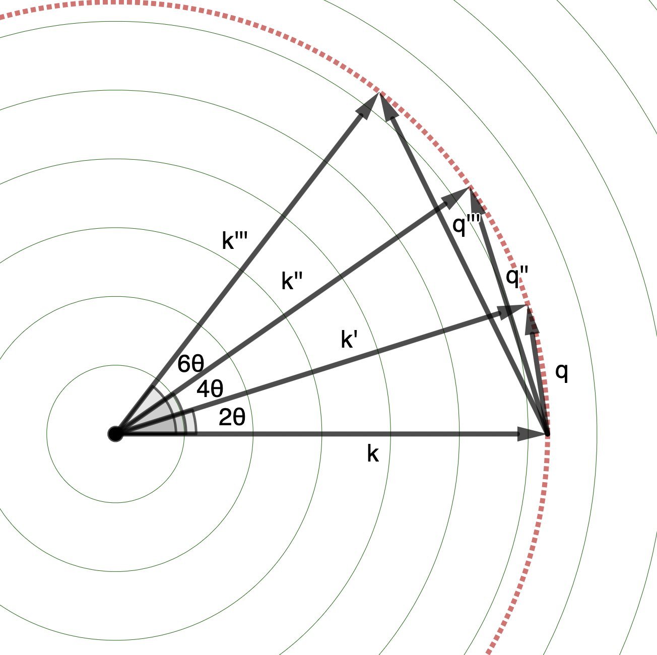
This intensity is a function of the “scattering factor”: \(\mathbf{q}\), which is vector displacement between the incident (\(\mathbf{k}\)) and scattered (\(\mathbf{k}'\)) wavevectors: \(\mathbf{q} = \mathbf{k}' - \mathbf{k}\).
The collection of these \(\mathbf{q}\)s forms a sphere in “reciprocal space”.
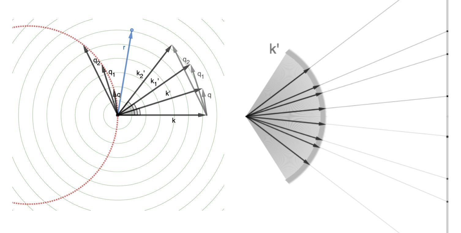
Because the magnitudes of both \(\mathbf{k}\) and \(\mathbf{k}'\) are \(2\pi/\lambda\), a smaller wavelength (\(\lambda\)) or higher frequency(\(f=c/\lambda\)) or higher energy (\(E=hf\)) X-ray beam corresponds to a larger radius for this sphere.
The “form factor” (\(F(\mathbf{q})\)) is the amplitude of the scattered X-ray beam, after all the effects of the scattering (constructive/destructive interference) are taken in to account.
It just so happens, this is equivalent to the Fourier transform of the electron density!
\[F(\mathbf{q}) = \int \rho(\mathbf{r}) e^{i\mathbf{q}\cdot\mathbf{r}}\mathrm{d}^{3} \mathbf{r}\]
The intensity (\(I(\mathbf{q})\)) we measure is proportional to the squared magnitude of the structure factor (\(\| F(\mathbf{q}) \|^{2}\)), which, it also just so happens, is the Fourier transform of the autocorrelation of the electron density:
\[\| F(\mathbf{q}) \|^{2} = \int [ \rho (\mathbf{u}) \rho ( \mathbf{r} + \mathbf{u} ) \mathrm{d}^{3} \mathbf{u} ] e^{i \mathbf{q}\cdot\mathbf{r}} \mathrm{d}^{3} \mathbf{r} = \int (\rho \star \rho)(\mathbf{r}) e^{i \mathbf{q}\cdot\mathbf{r}} \mathrm{d}^{3} \mathbf{r}\]
Now, so far, we’ve been dealing with the scattering through a general volume of electron density.
As I teased last time, things get much more interesting when we enforce that this density is periodic in space.
That is, that the electron density is organized in a crystal 💎!
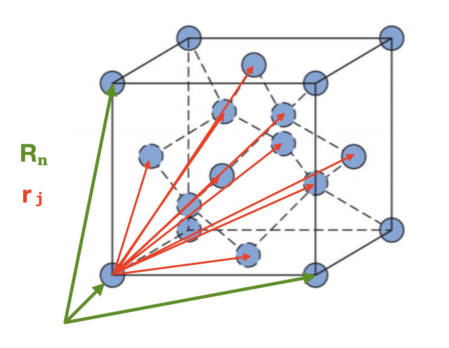
A crystal is a group of atoms arranged in a “unit cell”, which repeats in three-dimensional space, tiled one after another like lego bricks.
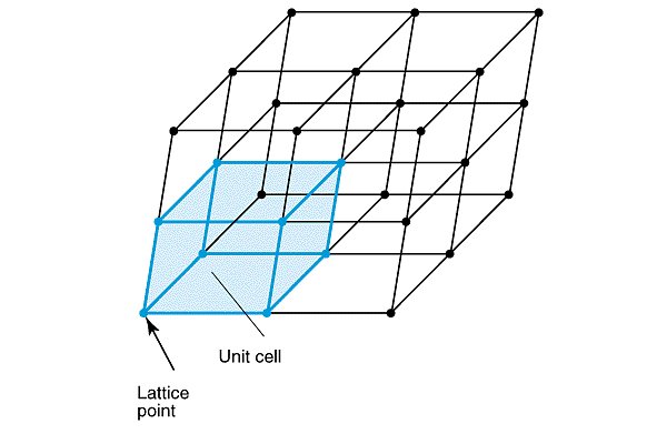
We can represent this mathematically by specifying the vector pointing to the origin of each unit cell (the “lattice point”s in the image above):
\[\mathbf{R}_{n} = n_{1}\mathbf{a}_{1} + n_{2}\mathbf{a}_{2} + n_{3}\mathbf{a}_{3}\]
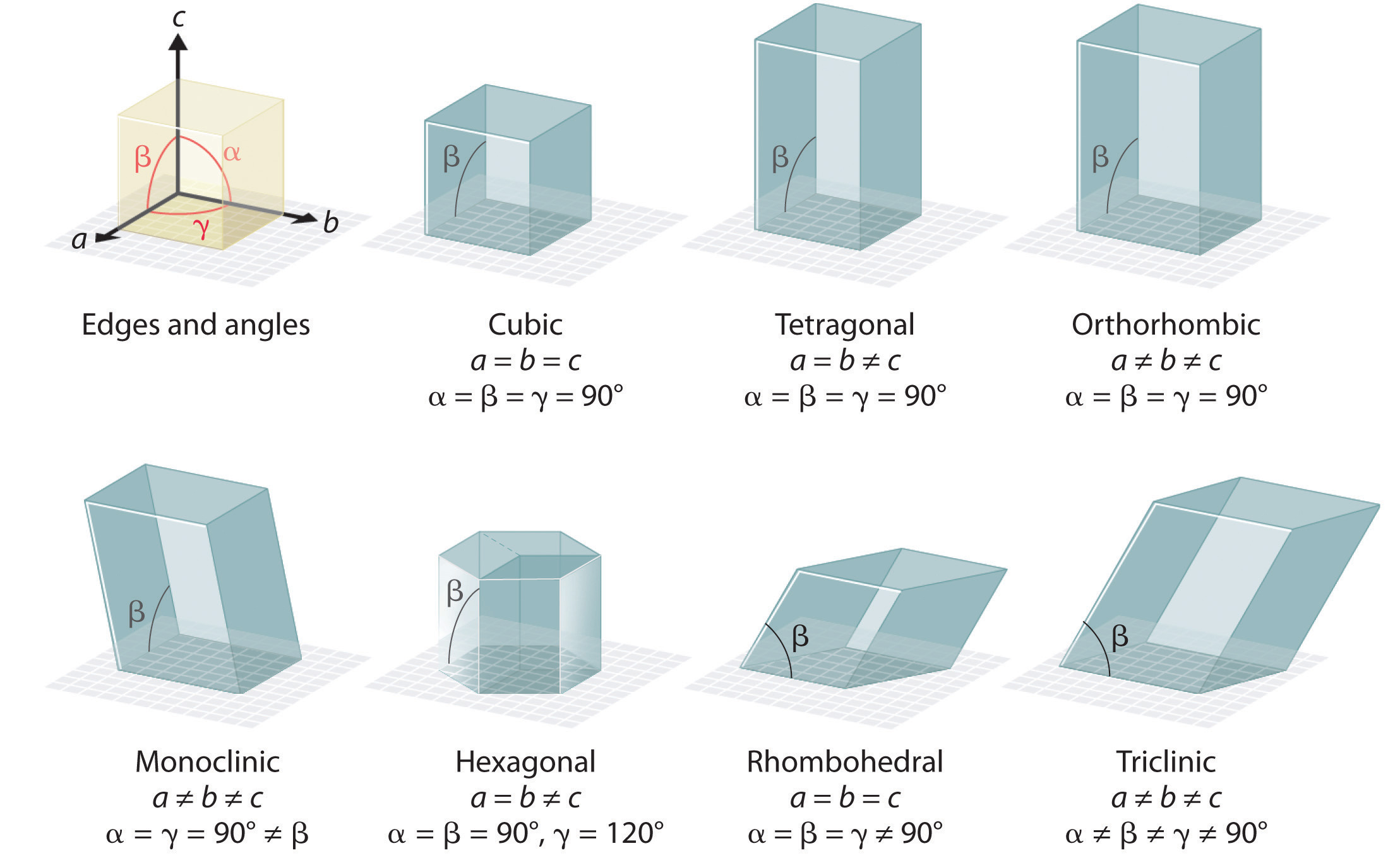
where \(\mathbf{a}_{1}\), \(\mathbf{a}_{2}\), and \(\mathbf{a}_{3}\) are the “lattice vectors” and \(n_{1}\), \(n_{2}\), and \(n_{3}\) are integers. (These are often notated as \(a\), \(b\), and \(c\), as in the image below.) Because we can define these unit cell vectors to point in any direction we like, we can describe all of the different types of unit cells found in crystals using the same formalism.
Now, because each unit cell is (theoretically) the same, we can specify the positions of all the atoms in the crystal, by specifying the positions of the atoms in the unit cells relative to each lattice point.
\[\mathbf{r}_{j} ⟶ \mathbf{R}_{n} + \mathbf{r}_{j}\]
Our form factor for the crystal is then:
\[F_{\text{crystal}}(\mathbf{q}) = \sum_{n} \sum_{j} f_{j}(\mathbf{q})e^{i\mathbf{q}\cdot(\mathbf{R}_{n} + \mathbf{r}_{j})}\]
\[= \sum_{n} e^{i\mathbf{q}\cdot\mathbf{R}_{n}} \sum_{j} f_{j}(\mathbf{q}) e^{i\mathbf{q}\cdot\mathbf{r}_{j}}\]
\[= \sum_{n} e^{i\mathbf{q}\cdot\mathbf{R}_{n}} F_{n}(\mathbf{q})\]
where \(F_{n}(\mathbf{q})\) is the form factor of the unit cell, relative to \(\mathbf{R}_{n}\).
Remember, though, this is not what we measure. What we measure (the intensity) is proportional to \(\| F(\mathbf{q}) \|^{2}\)!
\[\| F_{\text{crystal}}(\mathbf{q}) \|^{2} = \sum_{n} \sum_{m} F_{n}(\mathbf{q}) F^{\ast}_{m}(\mathbf{q}) e^{i\textbf{q}\cdot(\mathbf{R}_{n} - \mathbf{R}_{m})}\]
In a “perfect” crystal all unit cells are the same, so we could factor out \(\|F(\mathbf{q})\|^{2} = F_{n}(\mathbf{q}) F^{\ast}_{m}(\mathbf{q})\), but in a real crystal, things are dynamic!
Unit cells differ!
So, we move forward by defining the average form factor:
\[F_{\text{avg.}}(\mathbf{q}) = \frac{1}{N} \sum_{m} F_{m}(\textbf{q})\]
and our intensity (\(\| F_{\text{crystal}}(\mathbf{q}) \|^{2}\)) now has two components:
\[\| F_{\text{crystal}}(\mathbf{q}) \|^{2} = I_{\text{Bragg}}(\mathbf{q}) + I_{\text{Diffuse}}(\textbf{q})\]
where:
\[I_{\text{Bragg}}(\mathbf{q}) = \| F_{\text{avg.}}(\mathbf{q}) \|^{2} \| \sum_{n} e^{i \textbf{q} \cdot \mathbf{R}_{n}} \|^{2}\]
This is the scattering from a perfect crystal, with our \(F(\mathbf{q})\) from before replaced by the \(F_{\text{avg.}}(\mathbf{q})\).
(The second term, the “diffuse scattering”, is what I study! It’s the scattering due to deviations from the average, and so contains information about dynamics rather than just the average structure. It is much weaker, and harder to interpret, which is why I have a job.)
We can further simplify the equation for the Bragg intensity by writing things as:
\[I_{\text{Bragg}}(\mathbf{q}) = \| F_{\text{avg.}}(\mathbf{q})\|^{2} \| S_{n}(\mathbf{q}) \|^{2}\]
where:
\[S_{n}(\mathbf{q}) = \sum_{n} e^{i\textbf{q}\cdot\textbf{𝗥}_{n}}\]
is the “lattice structure factor” from the \(N\) unit cells.
Because the \(\textbf{R}_{n}\)s are all multiples of each other, at certain values of \(\textbf{q}\), \(\textbf{q}\cdot\textbf{R}_{n}\) will be \(2\pi\) times an integer and \(e^{i\textbf{q}\cdot\textbf{R}_{n}} = 1\).
This is basically just the “phase factor” (\(\Delta\phi\)) we learned about in Part 1, but for the whole crystal.
As we saw then, this is just a clever mathematical trick we use to identify the angles at which the scattered waves constructively interfere!
The value for the intensity at \(\textbf{q}\) then will just be \(1\) times \(F_{\text{avg.}}(\mathbf{q})\)!
So the Bragg peaks give us info about average structure!
Unlike a small collection of atoms, in a crystal, this constructive interference happens over & over again by necessity.
Because a crystal repeats in space, if \(\textbf{q}\cdot\textbf{R}_{n} = 1\) so will \(\textbf{q}\cdot\textbf{R}_{2n}\) and \(\textbf{q}\cdot\textbf{R}_{3n}\) etc.
This repeated constructive interference leads to strong peaks in the intensity at certain angles! We call these the “Bragg peaks”.
In fact – side note for the physics nerds – the X-ray beams we use are often basicaclly monochromatic, so the photons’ momenta are very precise. This means the photons positions are known very imprecisely, due to the Hiesenberg Uncertainty Principle. So, you can think about the photons as scattering off of the whole lattice plane at once.
It becomes advantageous, then, to define a “reciprocal basis”:
\(\textbf{a}^{\ast}_{1} = \frac{2\pi}{v} (\textbf{a}_{2} \times \textbf{a}_{3})\)
\(\textbf{a}^{\ast}_{2} = \frac{2\pi}{v} (\textbf{a}_{3} \times \textbf{a}_{1})\)
\(\textbf{a}^{\ast}_{3} = \frac{2\pi}{v} (\textbf{a}_{1} \times \textbf{a}_{2})\)
where these vectors (by construction) have the property that
\[\textbf{a}_{i} \cdot \textbf{a}^{\ast}_{j} = 2\pi \delta_{ij}\]
where \(\delta_{ij}\) is the Kronecker delta, and v is the unit cell volume \(v = \textbf{a}_{1}\cdot(\textbf{a}_{2}\times\textbf{a}_{3})\)
(For those unfamiliar, the Kronecker delta construction here just means that if \(\delta_{ij} = 1\) if \(i\) and \(j\) are equal and \(\delta_{ij} = 0\) if \(i\) and \(j\) are not equal – this ensures \(\textbf{q}\cdot\textbf{R}_{n}\) at the nodes of our new “reciprocal lattice”.)
We can now define the “reciprocal lattice” we just mentioned, as:
\[\mathbf{G}_{h} = h_{1}\mathbf{a}^{\ast}_{1} + h_{2}\mathbf{a}^{\ast}_{2} + h_{3}\mathbf{a}^{\ast}_{3}\]
where \(h_1\), \(h_2\) and \(h_3\) are integers – our “Miller indices”.
Because of the way we’ve set everything up, the Miller indices correspond to the exact places in reciprocal space where we get constructive interference from the crystal lattice!
\[\textbf{G}_{h}\cdot\textbf{R}_{n} = 2\pi(h_{1}n_{1} + h_{2}n_{2} + h_{3}n_{3})\]
So \(e^{i\textbf{q}\cdot\textbf{R}_{n}} = 1\) when \(\textbf{q} = \textbf{G}_{h}\) for integer \(h_{1}\), \(h_{2}\), and \(h_{3}\)!
This, believe it or not, is equivalent to Bragg’s law!
Our waves constructively interfere when the crystal is oriented such that we get scattering off of a lattice plane (defined, now, by our “reciprocal lattice nodes”).
Now, we have a way to represent everything we need in reciprocal space!
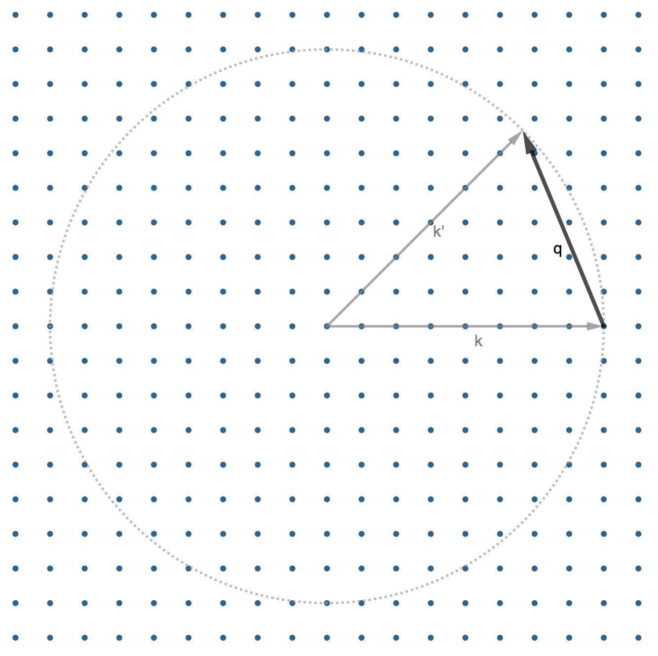
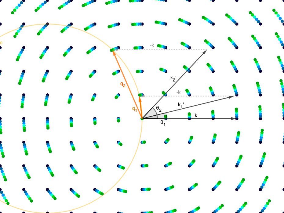
If we want to know when we’ll see constructive interference, or a “Bragg peak” in real space, we just need to find angle (\(\textbf{k}'\)) where our scattering vector (\(\textbf{q}\)) intersects a node of our reciprocal lattice!
We noted before that the collection of all the different angles we could diffract away from our incident beam forms a sphere of k’s and thus a sphere of \(\textbf{q}\)s (because \(\textbf{q} = \textbf{k}' - \textbf{k}\)).
This sphere is called the “Ewald sphere”!
We said: we measure (at the detector) in the \(\textbf{k}'\) direction, but the degree of constructive interference depends on \(\textbf{q}\).
Now, for a crystal, we know exactly how!
If \(\textbf{q}\) intersects a reciprocal lattice node, we get a peak in the \(\textbf{k}'\) direction on our detector!
This doesn’t always happen though: as you saw in the above image, the Ewald sphere only intersects a few nodes of the reciprocal lattice for each incident angle for the X-ray beam.
But guess what we can do?
We can ROTATE THE CRYSTAL!
This rotation then exposes the Ewald sphere to a different set of lattice nodes at each angle of rotation!
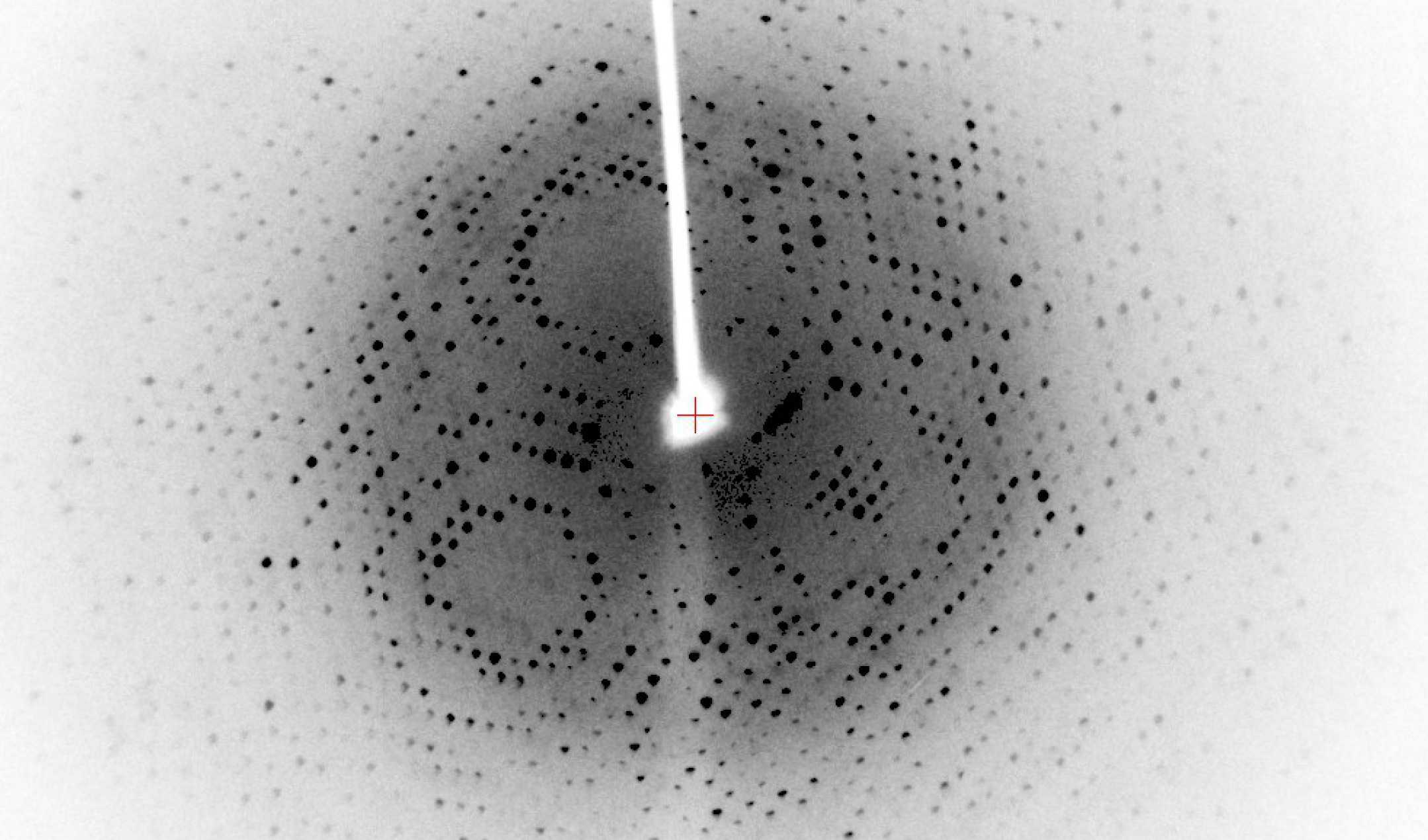
Now, you know everything you need to know to understand what’s happening in the video below, from a real protein crystal diffarction experiment.
This is a real set of images from experimental X-ray diffraction through a protein crystal.
Watch what happens as the crystal rotates:
At each different angle, the Ewald sphere is intersecting a different set of nodes in the reciprocal lattice, and that leads to a different set of Bragg peaks on the detector!
We collect the data on all the Bragg peaks, at all the different angles, and stitch them together to create a full 3-D dataset for the values of \(\| F_{\text{avg.}}(\textbf{q}) \|^{2}\) at every reciprocal lattice node.
This encodes all the information we can get about \(\| F_{\text{avg.}}(\textbf{q}) \|^{2}\) (the average structure).
Isn’t that just beautiful?
By constructing the right mathematical objects, we can represent what’s going on in experiment in a dual space, such that all the complicated physics gets compressed to a geometrical game of rotating a sphere so that it intersect nodes of a lattice.
One last thing, before I go:
Way early on, we noted that the magnitude of \(\textbf{k} = \frac{2\pi}{\lambda}\), so a smaller wavelength (higher frequency, higher energy) X-ray beam means a longer wavevector, \(\textbf{k}\).
This means a higher-energy X-ray beam sweeps out a larger Ewald sphere.
Thus, we can get information about a larger area of reciprocal space by hitting the protein crystal with a higher-energy X-ray beam. ⚡️⚡️⚡️⚡️
Because the spacing between reciprocal lattice nodes only depends on the size of the unit cell (they’re “fixed”) we can intersect more nodes of the reciprocal lattice at each angle of rotation for the crystal by collecting data with higher-energy X-rays!
Huge facilities have been constructed around the world, to spin electrons around at close to the speed of light, which radiate out high-energy X-rays that are then focused in to beams and sent through crystals of proteins (and other stuff).
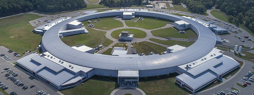
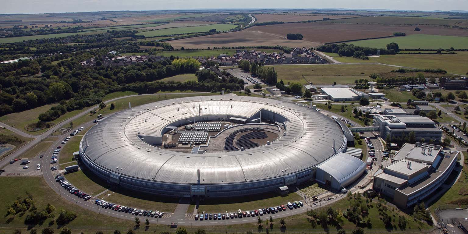
(Above, NSLSII at Brookhaven National Laboratory in the US and Diamond Light Source in the UK)
I hope to follow up at some points with a similar thread about the diffuse scattering.
For now, be well!